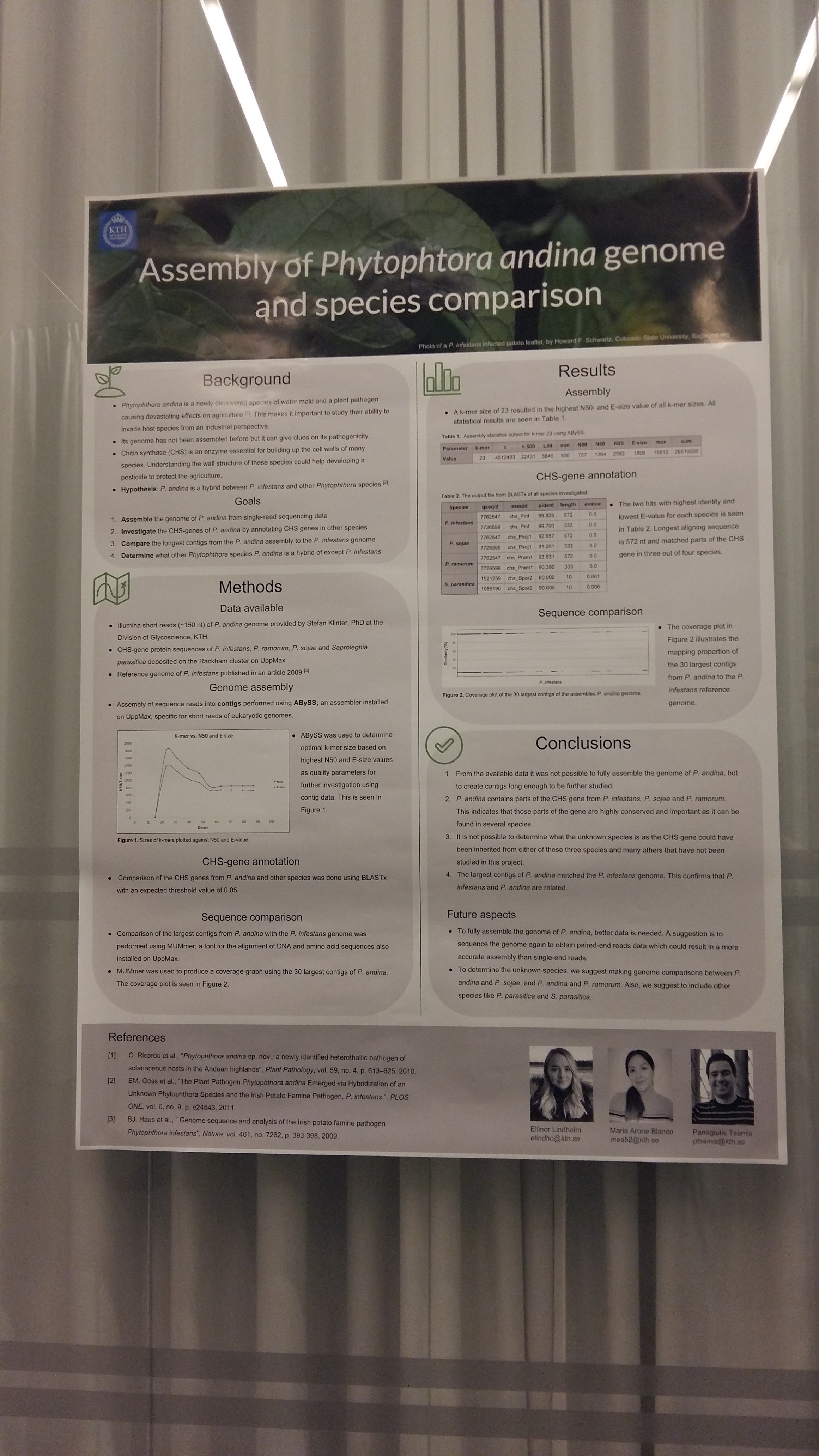
Yesterday we presented our poster at SciLife! It went very well and people seemed interested in our project. We were told several times that the poster was very appealing and one even said it was the best looking one, and for that we are very happy! Here is the poster as presented yesterday:

Our poster during the conference.

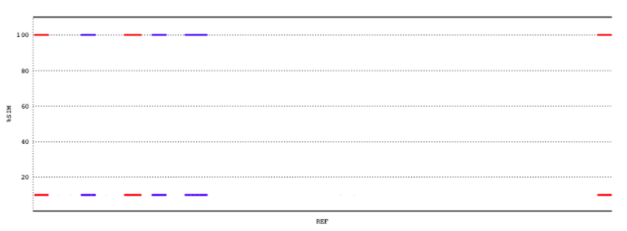
We noticed that what people found to be most difficult to understand was the coverage plot which we also struggled with to fully understand and to present in a good way with colours etc. But I think most understood after having it explained a bit extra. Other than that, there didn’t seem to be anything unclear about the poster or the project.

With that I think this is my last post and I want to thank Stefan Åhman for helping me with any issue I had with Github or uploading of posts, and Oscar He for giving advice to our project and tips. Additionally, I want to thank Lars Arvestad, one of the course teachers who helped us answering questions during the project and giving us feedback. Thank you!

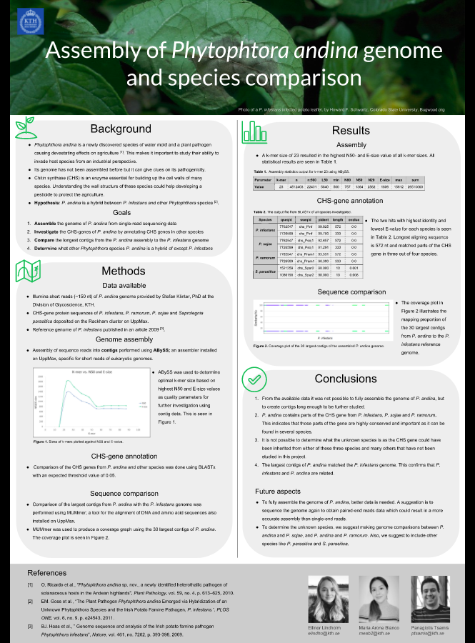
The final poster is ready and can be seen here (digital version):

Screenshot of the final poster.

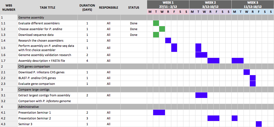
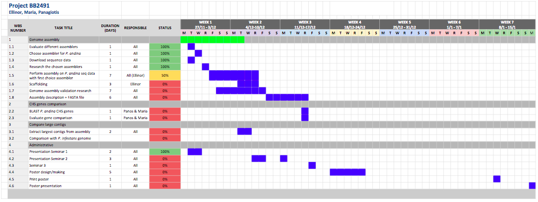
Today the poster was also printed in AlbaNova which means we are done with the last part of the project. The Gantt-schedule (having been revised very little) can be seen here:

Current Gantt schedule

We are really happy with the poster; both the content and the look of it. What remains now is talking through it, making sure we understand and know all the content before the poster presentation the 15th of January.

Below I have summarized our final conclusions.

• From the available data it was not possible to fully assemble the genome of P. andina, but to create contigs long enough to be further studied.
• P. andina contains parts of the CHS gene from P. infestans, P. sojae, and P. ramorum. This indicates that thsoe parts of the gene are highly conserved and important as it can be found in several species.
• It is not possible to determine what the unknown species is as the CHS gene could have been inherited from either of these three species and many others that have not been studies in this project.
• The largest contigs of P. andina matches the P. infestans genome. This confirms that P. infestans and P. andina are related.

As future aspects, there are two major points we want to mention.

• To fully assemble the genome of P. andina, better data is needed. A suggestion is to sequence the genome again to ibtain paired-end reads data which could result in a more accurate assembly than single-end reads.
• To determine the unknown species, wes uggest making genome comprisons between P. andina and P. sojae and P. ramorum. Also, we suggest to include other species like for example P. parasitica and S. parasitica.

Now we will prep for the poster presentation, and come back with feedback we get. See you there!

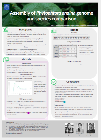
Since last time, our group has worked a bit on the poster, and it’s almost finished. Panos has, as I’ve mentioned in the last post, focused on finalizing the part where we are using MUMmer to compare the sequences and Maria has primarily helped me with the poster, writing texts and adding figures. We have also had a break over Christmas which was well needed.

A screenshot of the how the poster looks at the time of publishing this post.

Today we ran MUMmer again to create a coverage plot with different colours to be added to the poster. While it was running we worked on the poster and discussed what results we wanted to add and what conclusions to write.

After some feedback from Lars regarding the usage of MUMmer, and the plots it can generate, we seem to be on the right track. For the upcoming days, we will work on the details of the poster and also upload data on CANVAS including a genome assembly description and the final .fa-file for Lars (and whoever) to look at.

We have also e-mailed the final assembly to Lars with the relevant statistics. I will post once more with all of the final results and conclusions, after the exams, and when the poster is finished.

Since last post, and over the weekend, all CHS-gene sequences from all species have been annotated using BLAST. Additionally, MUMmer has been used to compare the largest contig with the published, assembled genome of P. infestans. Below are the results and some conclusions.

CHS-genes for all species

For all species, except S. parasitica, the best hits were sequences of length 572 and 333. This includes P. infestans as described in the previous post. The table below shows the top three hits for P. infestans, P. sojae, and P. ramorum.

The top three hits in BLAST for each species' CHS-gene sequence against the assembled genome of P. andina.

To conclude, the assembled genome of P. andina have contigs that match parts of the CHS-genes of all species, except S. parasitica. As the same sequence matches (as can be seen the longest matches are of exact same length), we have concluded that this sequence most likely is highly conserved between the species, but we cannot tell from these results from which species P. andina has specifically inherited this gene. We know P. andina is a hybrid between P. infestans and “other species”, and it is not too far fetched to assume that the “other species” could be all or some of these. However, we also cannot tell if P. andina is a hybrid with S. parasitica or not, just because they do not share this gene sequence.

In order to know more about the relatesness of P. andina to all of these species, we could instead of just comparing the largest contig from P. andina assembly with the genome of P. infestans, compare the largest contig to all species’ genomes. However, as of now, we do not know if these assembeld genomes exist and this is originally outside of the project’s scope. If more time was available, we discussed that one could compare all contigs of P. andina, individually with all other species’ genomes and investigate overall similarity.

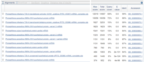
What we did was using BLAST against all for the largest contig. And the results can be seen in the figure below.

BLAST results of largest P. andina contig against all. E-value cutoff of 0.05 is used.

As seen here, P. infestans appears again, which is expected. However, seen is also a species called Phytophotora parasitica which was not included in the species we were asked to investigate. Therefore, it might be interesting to look into this species as well in the future.

Using MUMmer to compare sequences

In order to run MUMmer, the module was first added (it was already installed on UppMax). The goal was to compare the largest contig from our P. andina assembly with a relevant reference genome i.e. that of P. infestans as published in 2009.

Panos ran the following command:

mummer -mum -b -c AATU01.1.fasta contig1.fasta > comparison.mums

where:

• AATU01.1.fasta is the reference genome of P. infestans and contig1.fasta is our largest contig (notice that the format is now .fasta and not .fa, otherwise MUMmer won’t run)
• -mum computes MUMs, i.e. unique matches between the query (our contig) and the reference genome
• -b computes both forward and reverse complement matches
• -c outputs the query position of a reverse complement match relative to the forward strand of the same query sequence

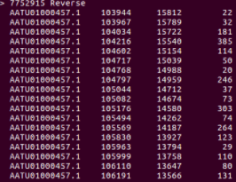
The screenshot below shows a small part of the output.

Output in the terminal after running MUMmer with the data and options as described above. For each hit, the columns represent the following from left to right: position in the reference sequence, position in the query sequence, and length of the match respectively.

In order to visualize the results, a plot was made.

mummerplot --postscript --prefix=ref_qry comparison.mums

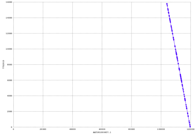
Where --postscript is the output format, --prefixis the first part of the output name, and comparison.mumsis the output file obtained from MUMmer. With this, we got three graphs. The output can be seen in the figure below.

Dotplot of the largest contig against the reference genome.

The y-axis here refers to the query sequence, which is the largest contig, and the x-axis refers to the reference sequence. At this point, we have concluded that is is a reverse complemented match (which is also expected) and this can be seen from its orientation. However, I find it very hard at the moment to assess the quality.

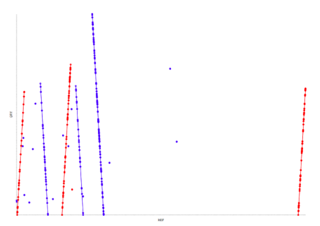
What we also tried was adding 9 more contigs, so we used MUMmer for the 10 largest contigs. It generated the following plot.

Dotplot with the 10 largest contigs against the reference genome. Only 6 contigs out of 10 have mapped.

In this figure, only 6 out of 10 contigs mapped to the reference sequence, with 3 of them mapping forward (red), and 3 mapping reverse (blue).

With the option -c, a coverage plot is obtained which illustrated the mapping of the contigs in a better way, although I would say we need more data for this to be useful, but I am not sure at the moment how this should look to be able to conclude valuable information from it.

Coverage plot of the 10 largest contigs against the reference genome. From now on, the goal is to produce a similar graph but with more data.

What we aim to do now, is adding even more contigs to get more data for a coverage plot. I will extract at least 10 more contigs and Panos will run MUMmer again. Maria have started working on the content of the poster, and I have started creating a design to it.

This is a long post as a lot have happened. Take your time!

Summary

Yesterday our group had a Skype meeting as we could not meet in person. We discussed what has been done since last time regarding the BLAST-part of the project, which is the following:

• All of us have used BLAST to annotate the CHS-genes against the assembled contigs using ABySS
• Panos has specifically annotated the P. infestans genes whereas me and Maria used all species’ CHS-genes.
• We have decided to continue with the dataset where a cut-off e-value of 0.05 was used (as allowing all e-values simply results in way too much data)
• The data have been sorted according to the order of p-identity, length and e-value
• We decided to first analyze the P. infestans data
• We decided that Maria continues with looking the BLAST results for all species we got genes for, Panos will update the assembly description and look into MUMmer, and I will also look into MUMmer and take out the largest contig from the P. andina assembly data.

BLAST results of P. infestans CHS-genes against assembled P. andina genome

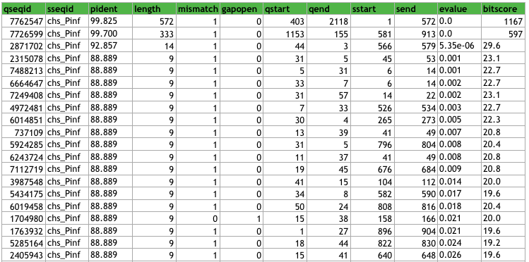
This is the top 20 rows of the P. infestans data sorted as mentioned above.

Top 20 hits after BLAST with P. infestans CHS-genes against assembled P. andina contigs.

When looking through the data, we can see that a lot of contigs overlaps (as expected), for example, the third hit (with length 14) represents a sequence that begins in the first hit (sstart = 3) and ends within the second hit (send = 579).

We can also conclude that the longest contig of the P. andina assembly in which a CHS-gene coding sequence from P. infestans can be found, is 572 bases long. However, note that this does not necessarily represent the longest contig.

BLAST evaluation

Here I will try to explain the parameters a bit and my view on them with regards to our results.

E-value

As mentioned, the parameters we look at are E-value, length that has aligned, and the identity. The E-value gives us information about the likelihood that the given sequence, i.e. the CHS-gene sequence, match purely by chance among our contigs. The lower the E-value, the less likely it is that the match was a result of a random chance, and the more significant it is.

For our two hits, the E-value is 0. To be honest, I initially thought the E-value approaches zero, but that it never can actually be 0, as this would mean there is no chance what so ever that it occurred by chance. I am not entirely sure why that can be at the moment, as there is “always” a chance (although infinitely small). Perhaps BLAST outputs 0 when the value is small enough, I will read into this more when I have time.

Anyway, what we can conclude with such E-values is that there is an extremely high confidence that the match is a result of a homologous relationship between P. andina and P. infestans for the CHS-gene, which is also expected as we knew beforehand that P. infestans was the closest relative to P. andina. It should also be mentioned that this is one of those genes that one can expect to be conserved over time between the species as it is vital for building up the cell walls, and thus we could expect to see these genes (and consequently chitin synthases) in most species with these type of cell wall structures and related phenotypes.

Identity and length

I think these two parameters are quite straight-forward, and the identity is very high for both hits, i.e. the extent to which the CHS-gene sequence have the same residues (and nucleotides) at the same positions is very high. For contig 7762547, it is 99.825%, and for contig 7726599 it is 99.700. For the contig 2871702, the identity is 92.657% which is still very high, but the length is very small and this contig is not really interesting for further analysis compared to one being almost 600 nt, although finding a much longer contig is ofcourse of interest for us.

Confirming contig sequence

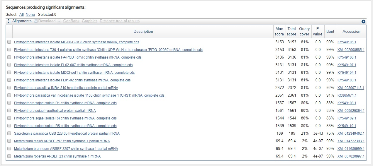
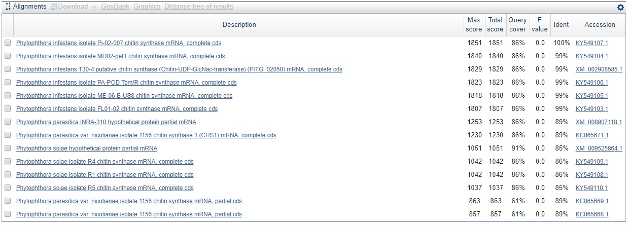
Just to test the contig sequence from the P. andina assembly that matched against the P. infestans CHS-gene sequence, we used the webbased BLASTn tool for the contig sequence against everything for all three hits 7762547, 7726599, and 2871702. The results can be seen in the three figures below.

Longest contig sequence (572 nt) for P. infestans BLASTed against all with blastn.

Second longest (333 nt) contig sequence for P. infestans BLASTed against all with blastn.

Shortest contig sequence (14 nt) worth looking into (based on the statistics parameters)for P. infestans BLASTed against all with blastn.

Not only have we confirmed that the sequence is indeed that of CHS-genes from P. infestans, but we can already here see that this sequence is found in other species as well. Perhaps most interesting is that the sequence is found with the same query cover and E-value, and just a slightly lower identity than that for P. infestans, in a species called Phytophtora parasitica which was not in our list of genes. This is also seen for the second hit which makes sense since the contig is part of the same gene sequence as seen from the sequence start- and end values, and knowing that the coding part of the P. infestans CHS-gene is around 2600 bp in total.

Longest contig for sequence comparison

To investigate the similarity between P. andina and P. infestans further, we will use MUMmer to compare the contigs against a genome of P. infestans that was published in 2009. To do this we need to take out the largest contig which is currently my responsibility of the project.

The .fa-output file from ABySS looks like this (10 first contig sequences):

>0 23 482
GCTGATCCTCGTGACTGTCGGCT
>1 23 79
CCTGACGAGCAGATCGGAAGAGC
>3 27 259
TCTATCGTCGAGGATGATCTCGACTTC
>4 23 11
ATCGCAATTTGAGCCACTCATAG
>5 23 5876
CTTTGGTGGTTTAACATTGTTTC
>7 23 29
TGAAGCTGCATTTGCTCTTGGTG
>8 24 86
GATCTATTGTATCACGTTCGCCAT
>9 26 565
AAGATATGTGTATCGAAAGAACCGTG
>11 24 9
CTTTGGTGGTTTAACATTGTTTTC
>12 26 271
ATAACGTGCAGCATCTTCAGGATGAA

For each sequence, identified with >, there are three numbers. The first one is the sequence id, the second is the number of bases, and the third is the number oh k-mers that were mapped to the sequence during assembly. Below is how the largest contig was obtained.

A regex helper function with gawk was defined to be able to take out a specific group.

$ function regex1 { gawk 'match($0,/'$1'/, ary) {print ary['${2:-'1'}']}';

Then, using regex, the sequence identifier (for example >12 26 271) was matched and the length of the sequences was sorted numerically.

$ cat assembled-unitigs.fa | regex1 '>[0-9]+\s([0-9]+).*' | sort -n > sorted-sizes.txt

The largest contig is found at the end of the output file sorted-sizes.txt.

$ tail sorted-sizes.txt
8584
8732
9157
9484
9690
9951
10148
10355
11835
15812

The largest contig is 15812 nt. This contig will be used in the next step to compare P. andina with P. infestans.

Planning ahead

Tomorrow, the 15th of December, we will have a meeting and go through the BLAST results as well as try and test MUMmerfor the first time. We will try and finalize the assembly description and the BLAST results as a whole, as well as discuss what our results mean for the project and the research in general. I am also glad that we are on schedule with everything that we have planned, and as it looks now, most of the work should be done in the middle of next week.

During Seminar 2 today, we presented the following presentation.

After listening to the presentations by other groups, it seems like we are in phase regarding how much we have done and how many tasks we have finished. We did not receive any feedback or questions, and since we have single reads, are project stands out a bit from the otherwise similar projects (for example there are two groups using ABySS, but they have paired ends).

Using BLAST to investigate gene sequences

Initially when using BLAST and testing different tools (specifically when using tblastn and tblastx) we got the following error:

Error message when using BLAST with the gene sequences and the contig-file obtained from ABySS

It seems like the error is due to the usage of a too large genome file (our contig-file from ABySS). So first we need to find a way to search for the genes in the whole file, or basically divide the file into several different files and BLAST them separately with blastx. Notice that this is when using the webtool.

When running it “locally” by first creating a database, it seems to be working. First, I created the database with the CHS-genes:

[ellinor@rackham3 Project]$ makeblastdb -in chs.fa -dbtype prot -out chs-genes-db

And three files are created: chs-gene-db.phr, chs-genes-db-pin, and chs-genes-db.psq.

Then, the following script is used with blastx and the contig-file as obtained with ABySS:

#!/bin/sh
# How to run:
# sbatch -A g2017020 -t 10:00:00 -p node -n 8 -o blastresults.out blast.sh

cd /home/ellinor/

# modules needed
module add bioinfo-tools
module add blast/2.6.0+

blastx -query assembled-unitigs.fa -db chs-genes-db -out chscontigsblast -outfmt 6

I decided to run all genes instead from just a few species as it’s very simple. But we will probably divide the analysis of the results between us. Notice that the output format is set to 6 as this should give just a simple, tabular output format which is easier to interpret.

The job is submitted on UppMax and running at the time of writing. I will update when the results have been obtained!

Weekly plan

We decided to have our next group meeting on Wednesday the 13th of December, and by then, we will have run BLAST and obtained results, as well as analyzing them. Me and Maria have run BLAST on all genes with -outfmt 6while Panos has run on only the P. infestans-genes with -outfmt 5. We also decided to look into MUMmeron Wednesday and perhaps continue and Friday depending on if we have problems or not

Since the last time, we have used ABySS to assemble the single read data of P. andina, with several different k-mers, and looked at the N50 and E-size values to somewhat determine the quality of the contigs.

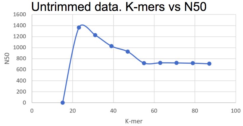
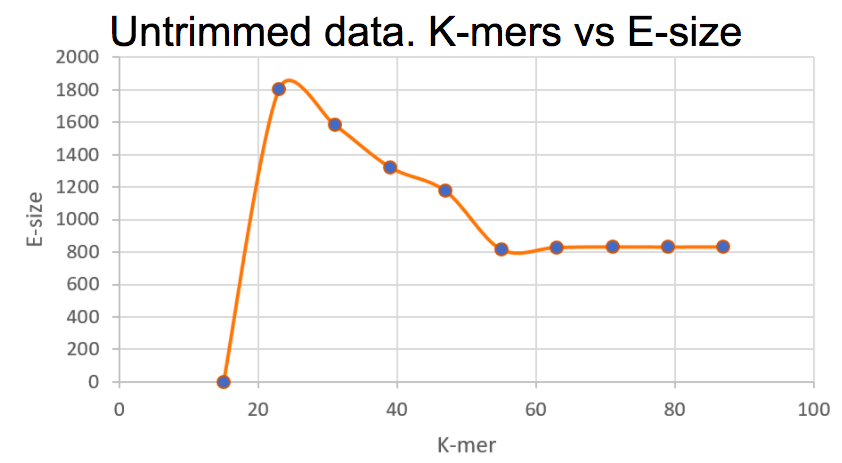
Below is two graphs where the k-mer sizes have been plotted against N50 and E-size, respectively.

Different k-mer sizes plotted against the corresponding N50 values. The highest N50 value corresponds to a k-mer of 23.

Different k-mer sizes plotted against the corresponding E-size values. The highest E-size value corresponds to a k-mer of 23.

Based on what we see here, using a k-mer of 23 seems like the best option for now. We did not see any difference in these parameters for the trimmed data using the tool sickle. After meeting with Lars Arvestad today, this is one of the things we brought up, and as we understood it, the data has already been trimmed from e.g. adapters, and therefore trimming it again does not make any real difference.

After the meeting, and after explaining what we had done so far and the results we had obtained, we could conclude that the assembly is more or less done and that the scaffolding part indeed is not possible as expected (since we do not have paired reads). The purpose of our assembly is therefore not to 100% assemble the whole genome, but rather to create contigs large enough for a whole genes to fit inside it, and hopefully those will be the CHS-genes. The problem with not being able to access the CHS-gene files was also solved during the meeting as Lars gave us access.

During a group meeting after the meeting with Lars, we sat down and started preparing the presentation for Seminar 2.

In this presentation we have focused on the three main tasks that define the project, and also what we have done so far and some issues that we have had. The presentation is not finished at the time of writing as we will work during the weekend and probably add more results.

To conclude what we have done so far in the project:

• Assembled the P. andina reads into contigs
• Evaluated which size of k-mer that gives highest N50 and E-size values
• Further defined the project and what tasks we have left
• Obtained and looked at the CHS-gene files. I though it was going to be DNA-sequences, but it was protein sequences which means we will just have to use the tBLASTn tool.
• Further divided the work and almost finished the Assembly description (one of the deliverables of the project).

Upcoming days

The main goal is now to finish Task 2 which is the identification of CHS genes. The CHS-gene file contains genes from four different species (all possible hybrids with P. andina):

• P. infestans
• P. sojae
• P. ramorum
• Saprolegnia parasitica

>chs_Psoj1 Phytophthora sojae
MSGAPPPSSGFAPRSYGQQPLSHAPRSSMMSVEYDGIPLPPPSIRSCGSQQYVTSYIPTGAAFPPSSVQDMISSMKSYASATDLVRTYSEIPSVEEALSTLDRAAAALNARRYRDALKLYLEGGYAMANVAERQANPKICNLLTSKGFETLNWCARLCDWIEGRIKEKHPRPGVHKVGIPVSNWDEDWVGPFMDEEEARRMWYTPVYCPHPIDFSNLGYRLRCVETGRRPRLMICITMYNEGPQQLKATLKKLANNLAYLKEQMPGDEKSLTGAFAGDDVWQNVLVCIVADGREQVHPKTLDYLEAIGLYDEDLLTINSAGIGAQCHLFEHTLQLSVNGKCLLPIQTVFALKENKASKLDSHHWYFNAFAEQIQPEYTAVMDVGTMLTKSALYHLLFAFERNHQIGGACGQLTVDNPFENLSNWVISAQHFEYKISNILDKSLESCFGFISVLPGAFSAYRYEAIRGAPLDAYFQTLNIELDVLGPFIGNMYLAEDRILSFEVVARKNCNWTMHYVKDAVARTDVPHDLVGLISQRKRWLNGAFFATLFSIWNWGRIYSESKHTFVRKMAFLVFYVYHLLYTAFGFFLPANLYLALFFIVFQGFQQNRLEFIDTSEYSQTVLDCAVYIYNFSYLFGLLMLIIIGLGNNPKHMKLTYYFVGAVFGLMMMLSSLVGAGIFFSTPATVHSIVVSILTVGVYFIASALHGEVHHIFMTFTHYTALIPSFVNIFTIYSFCNLQDLSWGTKGLHDDPLLAASLDETEKGDFKDVIAKRRALEELRREEKERVENRKKNFEAFRTNVLLTWAFSNLIFALFVVYFASSSTYMPVLYIFVASLNTCRLLGSIGHWVYIHTEGLRGRVIDKSECGNGTGRYPQNSYVQLEEHYAALAEDQRTYASGRTNASVRTVNDVSSAA
>chs_Psoj2 Phytophthora sojae
MEQDGGGYVSSNAEEYDAAPSSGLPTPDGPDVWRDTRPTSHSYVDEPHANQPIERQLSYRQPGLNPAAEETYEAAFRLIQLAADAERSGSPLQAIQLYTDAGDVLIKVGKREPDPLLKQGIRQKANEIMKRAEELDEWYYSVQESARKAALPPQLQIQRTQVPRVQEAWQGRKPTLSQAPEFTHMRYTAVSTKDPVKFSDDGFQLRVEEAGKKIRVFITITMYNEEGSELQGTLKGIARNLEFMAEQWGDRAWESVAVAVVSDGRTKASASCLDFLAGLGAFDEEIMTVTSMGVDVQLHLFEATVQLVRDDNFESFYPPIQLIYALKENNAGKLNSHLWFFNAFSEQLLPTYTVLVDVGTIPGPTSIFKLIRSMDRNPQIGGVAGEIAVDHPNYFNPVIAAQHFEYKISNIMDKSLESVLGFISVLPGAFSAYRYEAIRAEKGVGPLPEYFKSLTTSTRDLGPFKGNMYLAEDRILCFELLARRGRNWTMHYVKDAIARTDVPETLVDLIKQRRRWLNGSFFAGLFAISNFSRVWKESGHSLSRKIVLTLQFIYLSVQNVLSWFLLSNLFLTFYYVLTLTLYSKYPALLAIVLGIYLAIVGGIVVFALGNRPEKRTAAFYSFSYVFMGLVMLVVSVISIYGLVADVSVTDPRDDLASCSVSNFELVGGVVTAIGLVFASAFIHGEFSVLLSTLQYYFMLPTFVNILGIYAYSNLHDLSWGTKGLETAGHGAAKVAQGNGNLKEIVAQQKRIEAEKQRAAQEKEDVDNSFRAFRSSLLLFWLVTNAVWMYCMTYFVSSSCYLKFISYVVAVFNVVRFFGSAVFLCFRIARRLGTCGASRSGKSGRNYQAHLPAEWQAHYKRSSNATTETTTTGNGQQTYVGLNISDLSSPAATNYRNMEEVR
>chs_Pram1 Phytophthora ramorum
MSGGPPPSSGFVPRSFGLPPISQAPRSSMMSVEYDGIPLPPPSIRSCGSQQYVTSYIPTGAAFPSGSVQEMISSMKSYASATDLVRTYSEIPSVEEALVTLDRAAVALNARRYRDALKLYLEGGYAMANVAERQANPKICNLLTSKGFETLNWCARLCDWIEGRIKEKHPRPGVHKVGIPVSNWDEDWVGPYLDEEEARRMWYTPVYCPHPIDFSNMGYRLRCVETGRRPRLMICITMYNEGPQQLKATLKKLANNLTYLKEQDSGHDKALSETFKGNDVWQNVLICIVADGREQVNDKMLDYLEAVGLYDEDLLTINSAGIGAQCHLFEHTLQLSVNGKCLLPIQTVFALKETKSNKLDSHHWYFNAFAEQIQPEFTAVMDVGTMLTKSALYHLLFAFERNHQIGGACGQLTVDKPFENLSNWVISAQHFEYKISNILDKSLESCFGFISVLPGAFSAYRYEAIRGAPLDAYFQTLNVDLDVLGPFIGNMYLAEDRILSFEVVARKNCNWTMHYVKDAVARTDVPHDLVGLISQRKRWLNGAFFATLFSIWNWGRIYSESSHTFTRKVAFLVFYGYHLLYTAFGFFLPANLYLALFFIVFQGFQQNRLQFIDTSDFSQTVLDCAVYIYNFAYLFGLLMLIIIGLGNNPKHMKLTYYFVGAVFGVMMMLSSLVGLGIFFSTPATINSIVVSILTVGVYFIGSALHGEMHHIFMTFTHYTALIPSFVNIFTIYSFCNLQDLSWGTKGLHDDPLLAASLDETEKGDFKDVIAKRRAMEERRREEKERTDNRKKNFEAFRTNVLLTWAFSNLILALFVVYFTDSSTYMPILYYFVASLNSCRLLGCIGHWVYIHTDGLRGRVLDKTECGNGTGRYPQNSYIQLDEHYAALVEDQRTYASGRTNASVRTNNDISSAA
>chs_Pram2 Phytophthora ramorum
MSNGRSTEDLRARLQSLRASRTSSLQPQEAARDWGDTFQPGELEELQSMLEQDAAGDFSSGTEEYDAIASSGLSTPDNVDVWRDTRPTSHSYVDEPHPNQPIERQLSYRQSGLNPAVEETYEAAFRLIQLAAEAERSGTPLQAIQLYTDAGDVLVKVGRREPDPLLKQGIREKANEIMKRAEELDEWYYSVQESARKAALPPQLQIQRTQVPRVQEAWQGRKPTLNQPPEFTHMRYTAVSTKDPVKFTDDGFQLRIEQAGKKIRVFITITMYNEEGSELQGTLTGIARNLEFMAEQWGDRAWESVAVAVVSDGRTKASASCLDFLTGLGAFDEEIMTVTSVGVDVQLHLFEATVQLVRDDNFESFYPPIQLIFALKESNAGKLNSHLWFFNAFSEQLLPTYTVLVDVGTIPGPTSIFKLIRSMDRNPQIGGVAGEIAVDHPNYFNPVIAAQHFEYKISNVMDKSLESVLGFISVLPGAFSAYRYEAIRAEKGVGPLPEYFKSLTTSTRDLGPFKGNMYLAEDRILCFELLARRGRSWTMHYVKDAIARTDVPETLVDLIKQRRRWLNGSFFAGLFAISNFSRVWRESGHSLSRKLVLTLQFVYLGVQNLLSWFLLSNLFLTFYYVLTLTLYSDYPVLLAIVLGIYLVIVGGIVVFALGNRPEKRTAAFYSFSYVFMGLVMLVVSVISIYALVADISVTDPRDDLASCSVSNFELVGGVATAIGLVFASAFIHGEFSVLLSTLQYYFMLPTFVNILGIYAYSNLHDLSWGTKGLETAGHAAAKVTQGNGNLKEIVAQQKRLEALKQRAAEEKEDVDNSFRAFRSSLLIFWLVTNAVWMYCMTYFVSSSCYLKLISYVVAVFNMARFLGSAVFLCFRIARRLGACGTVRSGASGRNYQASLPIEWQAHFKHSSNTTTETTTRNGHIGLNMSDLSSPVATNYKNMEEAM
>chs_Pinf Phytophthora infestans
MSGAPPPSSGFQPRSIGLPPLSHGPRSSMMSVEYDGIPLPPPSIRSCGSQQYVTSYIPTGAAFPSGSVQDLISSMKSYASATDLVRTYSEIPSVEEALVTLDRAAVALGARRYRDALKLYLEGGYAMANVAERQANPKICNLLTSKGFETLNWCARLCDWIEGRVKEKHPRPGVHKVGIPVSNWDEDWVGPYLDEEEARRMWYTPVYCPHPIDFSNMGYRLRCVETGRRPRLMICITMYNEGPQQLKATLKKLANNLAYLKEQKKDHEKTLSRDFAGDDVWQNVLLCIVADGREQVNDKMLDYMEAIGLYDEDLLTINSAGIGAQCHMFEHTLQLNVNGKSLLPIQTVFALKESKSSKLDSHHWYFNAFAEQIQPEYTAVMDVGTMLTKSALYHLLFAFERNHQIGGACGQLTVEKPFENLSNWVISAQHFEYKISNILDKSLESCFGFISVLPGAFSAYRYEAIRGAPLDAYFQTLNIDLDVLGPFIGNMYLAEDRILSFEVVARKDCKWTMHYVKDAVARTDVPHDLVGLISQRKRWLNGAFFATLFSIWNWGRIYSESNHSFTRKMAFLVFYLYHLLYTAFTFFLPANLYLALFFIVFQGFQQNRLEFVDTSEYSQTVLDCAVYMYNFVYLFGLLMLIIIGLGNNPKHMKLTYYFVGAVFGVMMMLSSLVGMGIFFSTPATTHSIVVSILTVGVYFIGSALHGELHHIFMTFTHYTALIPSFVNIFTIYSFCNLQDLSWGTKGLHDDPLLAASLDETEKGDFKDVIAKRRAMEERRREENERMENRKKNFEAFRSNVLLTWTFSNLIFALFVAYFADSSTYMPILYIFVASINSCRLLGCIGHWIYIHTTGLRESFLDKSECGNGTGRYPQNSYVQLDEHYAALAEDQRTYASGRTNASVRTNNDVSSIA
>chs_Spar1 Saprolegnia parasitica
MPPKRPTEASGRRYAPPAGRPSNNAANAKPRAPRKGVSSRASNVPSAASSYEYDYEYNMMPMMQAPPKSQPTFLSNIAPISAKEASMKGSNAMQLLLQGTSFTIDDAFRAIERAIQAENEGRFREALKHFLDGGEMIVTAAEKEASQKVRNLLLHKGKEVLEWAEHLAEWIERYNTSTPPVRIAKPMAVEVTYDRTMNSPDLDETEARMMFYTPVCSGPKAFTETGYRLQCIQSGRRPRLMVVITMYNEDENELRSTLRKVCNNVLYLKQHSLPGYEGDDAWKQVLVVVVSDGRTKANKGTLEWLANVGLYDEDVMNITSTGVKVQCHLFEHSLQMTKENSIRFPPLQLDSHLWYFDAFAEQIMPDYTVLLDVGTMPTKSSFYKLLTALEINAQIGGVCGEIAVDKPLPNMCNWVIAAQHFEYKISNILDKSLESCFGFISVLPGAFSAYRYKAIRGAPLQAYFKSLTTDMAELGPFAGNMYLAEDRILCFELLARKDCNWTMHYVKDAIARTDVPTNLIDLVGQRRRWLNGSFFATLFAIWNWGRVYTESNHSLTRKLALLVHALLGVSAANFYLALYFVIFQGFRDNRWNFIDTSEYPQWVLDGLPTAFNVFYAVTVFTQVTIGLGNKPKHVKGTHYLISVLFGLLMLLASGVAIVIFITSSKDAMAIVLAVLILGTFFIGSALHCEVHHIVLTFVQYTALMPSFVNILMVYSFCNLHDLSWGTKGIDTGHEAHKTEAVGQYKDIVARQKALEAKKAQDARNQDELKKRFDSFRSNLLLVWVMSNMSMVIICVNTVGADSFLPFLYAFVAAFNGIRLLGCIGYLIYYARQFLLFNTLSATGVLHKRHEARKHKKAEDPDPIDMELGTFNEPATSEIGAPMMQAPYNRMR
>chs_Spar2 Saprolegnia parasitica
MSDSNLDLAARLRALREGGAEPAPAPAPTPYMHSPPSRTRPTPLYTQESLEFGGTYTTGSPVGAEADGVYTQVPVWKDSKEKTYGYLDDEPAPQAQTLLNKANDLVQRQASNKAFRRQHTAAFRPLPNTVEELLDGSPTYEGAFRLVQLAVQMEQDGDPQAAINLYADAGATLVEVGRKEVDPLLQKGIRQKAQELLQRAEDLEAWMNGVAEEARKAALPPSLRIARTNVPTVEQTWAGRPPPFHDANEFKLMRYTAVATKDPIQFSDDGYVLRVHELQRPIKVFITITMYNEEGSEIKGTLTGLAKGLAYMCKEYGDDFWQQVAVAIVSDGRTKASKTCLEYLKAVGAFDEEIMTVTSLGVDVQMHLFESTLQLVENQNFEAYYPPLQVIYALKENNGGKLNSHLWFFNAFSEQLNPKYTVLVDVGTIPAETSVFRLIRSMERNAQIGGVAGEIAVEAPNFFNPVIAAQHFEYKISNIMDKSLESVFGFISVLPGAFSAYRYEAIRAVKGVGPLPEYFKSLTSTTKELGPFQGNMYLAEDRILCFELLARKQRRWTMHYVKDAIARTDVPETLVDLIKQRRRWLNGSFFAGLFAIGHFGRVWSQSSHSFGRKLVFTFQFVYLALQNLLSWFLLSNLFLTFYFVLTLAFTESAPALLQTMLTVYLAIIGGLIVFALGNKPEPRTASFYLFSCLYMGIIMLLVTGISIYGLIGKGTSAVKDPRTITGIFSNCTVSDAELAGGVITSLGLIFLSAFVHGEFGILLSFVQYFFMLPTFVNVLGIYAYSNLHDLSWGTKGLESGGGHGPAKAGGGNVKDVVEQQKKIEAARQAAAREKEDVDNSFRAFRSTLLLSWLTTNGIWLYVVTDYMSSGCYLKGLSYIVGFFNVVRFTGCVVFVILRMFRRFGCGARASRDNYQEALPAEWQTHYNVTNRTDGRVAPPPKHAASMDPTTPHGGVYQQV
>chs_Spar3 Saprolegnia parasitica
MGVPTLSKASVFRFARQPRHHGVKTRLLRSRSKTLMLGGQSTAETAQYASCNPNGDETSSNSLKPLKLKDMSTDDLLRHAEQLDMHLAKIYIESQKTKALAPIVTKSIGLPQQLWEDAGVAPPYHSAAEFQDLRYTAVRTADPIAFSADGYSLRVHTLGKSIKVFITVTMYNEPASQLQATLTGLAGGIDYLCHQYGYDFWQEVAVVVVADGRSKTHHSVLPYLESFGAFEKNLLAQAIAASKDTHVHLFESTIQLRKTNGSFHAPMQLIFALKEHNAGKLHSHLWFFNAFSEQVDPTYTALVDVGTVPAESSVYRLIRSMERNPQIGGVAGEIAVDDPDFFNPVIAAQHFEYKIANIMDASLQSVFGFIGVLPGAFSAYRYEAIRPINGVGPLAEYFKSLTASKKELGLCVGNMYLAEDRILCFEILARKNCDWTMHYVKDAIAHTDVPETLVDLIKQRRRWLNGSFFAGLFAIWNFGRVWTQSAHSLPRKCAFSLQFLYLAFQNVMNWFLLSNLFLTFFYILSLALYYKSIELLHVVLGTYFVLVGSLIVFALGNKPGHRTAIYYRVSSYIMGTIMLCVTCISLYALLGNVQFVDPRSDLPSCSVSNYELEAGAFFSLGIIFVCAFMHGEFGIVRSTVQYFFMLPTFVNVLGIYAYSNLHDLSWGTKGIETSAGHNGLPTSKFGSVKDMVALHLNATSTTDVVSEADKRKGVVAAEHEDVDNRFRVFRSLLLLTWLLTNGCWLYYATSFISCSCYLKYLSYIVAVFNTFRFLGGLLFLSFRMARGALHCCRQGVKKTRPLRCGNPQAGDDCSPV
>chs_Spar4 Saprolegnia parasitica
MTTLPERLLARVTSSMSALGGTAKLVTAQEGFRLIEQGVLAERQQHYKEAVDRFLGAAGVLDAVAATEADLHVRRLLHAKASDVVAWTEGIVAWMQHRPEVRPAYPPRQSKGISMPTTTVSAATLAFGMDEVERTSLHYTPVLTRSPSEFSRDGYELQVLRRHRRPRMLIVITMYNEDGSEIEATLRKVGNNVAYLCRHDLPGYEGELAWQNVLVVIVSDGRAKASASTLITLREMGVYDEDTLRITSAGLATSMHLFERTLLLPEAPGAKKLWTHTSETMPPLQVVFALKEENAGKLHSHLWFFHGFCNQVDPTYTVLLDVGTLPTKSALYKLVSAMEVNQQVGGVCGEIAVSQPLPHLTSLIISTQHYEYKISNVLDKATESCFGFISVLPGAFSAYRFKAIQGAPLDAYFKSLTTDMLALGPFQGNMYLAEDRILCFELLARKNCSWTMMYVKDAIARTDVPTTLVDLMAQRRRWLNGSFFAMLYTIFNWGRVYSEARHSLCRGLALLVQYTFMTVQVVFNWFLVANFYLTVYYVIFYALERNALGVLDTRAFYASHGALAKGLFNVVYGLVFVVQIILGMGNRPKHVARTYRAIGAYYMLLVVLTTAASVLTLVHTGAAALAPKEIALGIAVFGVYFIAAACHCELHHIVLSFVQYSLLLPVMINTLTIYSFCNLQDLSWGTKGIDTSSHDTGASENGEYKDVVARQKAAEDRAKQAAATTDLVRRRFDSFRSNLLLLWLVSNAALVGGLLYGALLDVYLPCLFVAIGAFNTYRLLGSLLFLLYTGRQWLLLQLCLCCGCLRRRYDRERRRGSDDRTMAILSPRDPLATI
>chs_Spar5 Saprolegnia parasitica
MVSSQLSTGLPAIARRPSVRSTRVGSHVRNDNDCVTTVDAFRYIERGVRAEYDMFYSEAINCFVNAGECLLIVAEQNDDDVSQMLLAKSQEVIGWAEELSIWLENGRAGPLPSRNCRGIQIPFTKEYEGGEHYEEAAELSYTPVATVNPINFTLDGYRMQCVTRGRKPTMMLVITMYNEDGAELAQTLRKVCNNVKYIQKNALPGYEGDDAWQNIVVCIVSDGRTKANPSATSFLRDIGVFNEDAMTIFSSGAATQMHLFERTVRLAKDPLNKQSVIMSNNSTIGADYPPLQMVYALKEHNAGKLNSHLWFFNAFCNQVDPEYNILLDVGTLPTKAALYKLLATLEMKADIGGVCGEIAVSRPIPNLWNFVIATQHFEYKVSNLLDKATESCFGFVSVLPGAFSAYRFAAIKGAPLQAYFKSLTTDMAELGPFYGNMYLAEDRILCFELLARTNGAWKLKYIKDAVARTDVPSTLVDLMAQRRRWLNGSFFAMLYSIVQWGRLYSHTNHSLFTKAGLLIQYFQLLVQLFFGWFMCGFFYLSVYYVVFTTLKKSKLPFWDSEEWYDDHHSMAMSIFNIVYAFLIMVQIIFGLGNKPKHVKWLYTFLSIFYAIVVITAVFFSVCSLSSHNGMSSFNIVLLAATFGVYFIAAAFHFELHHVVFTFVQYLVMLPTTINILMIYAFCNIQDLSWGTKGLGDSAGHGPTKGGGQRLGSGGYSDLVAQRKAAEAAARHDAVVADQVRRRFDSFRSYTLLFWLISNALLIMTCIYFVGANVFLPSLFLFIALFNVTRLLGSIAFVLATGRDWLLLKLCLCSGGMAKRKQKKEKVKDQDGFGALDSSKVLRHSA
>chs_Spar6 Saprolegnia parasitica
MSRRNYAPAARGGNGPRPNMNPANMGPPPQMPPPQHGSGRNLRAPPPRQVQQQGSFDRDSDDDMYGQHGANGVLGVPVWQDSAAYEHGSYLQENTPPSQRIPYPGPQGGGMMPPPGGMMPPPQQFAPAPVRMLNAGALQNQSNQQMQVMRDSNVGQAVPASTPEAFRIIASGVTAEAEARYQSAVNDFLAGGEMLALVSEREADPHIRSLLNTKAIQVLEWSKNLHDWYQQGMRGPMPRRFVGKIGVNVVNRLGACAGRIDAGSPSELRTMYYTPAANKVVSDFTKDGYRLQCIEEGRTPQLMVVITMYNEDQVEMYSTLKKVANNIAHIKSQKLPGYEGDDAWKNILVVIVSDGRTKANKGTLAFLRDVGAFDEDVMNILMVGVDVMCHVFEFCVQLKKANTIEASASSSERYPPTQVVFALKEHNGGKLNSHEWYFNAFAEQIQPEYTVLLDVGTMPTAKAFYLLLCAMEIDPQIGGTCGEIAVDKPIPHLCNWVIAAQHFEYKISNVMDKSLESVFGFISVLPGAFSAYRYKAIRGAPLEAYFKSLTTPMNELGPFQGNMYLAEDRILCFELLARRNCRWTMQYVKDAIARTDVPTDLVALIGQRRRWLNGSFFALVYTILNWGRVYTESNHSYIRKFFLCIQYAYMTANVALSWVLPANFFLVTYFLVIVGFKQNNWGYIPTSGIPENTKDIIVQVFSLLYGTSFLIQLVAGLGNKPKHIKGVYRLTAVFYALVMLLTSVIAFGFIMKPWIDSLRSGVPFAAMVTSFEIKDIAAFVASVGVFFLASCLHCEMHHIAMSFIQYMCLLPTFVNILNTYSFCNLHDLSWGTKGLESSDGHGPKAGGGGNYKDAAEAKKAEEARKKKEGEIKDKMEGDFQYFRSKLLIFWLLSQMGFAYLIISFDSVNGQEGANYLKFLFYIVAGFNLFRLFGSTYFLLIEARICVEKMCIRGTMRDRLKAKKKKQAIRAAQTQHV

For the next meeting, which will take place on Monday the 11th after Seminar 2, we plan to have done the following:

• Panos will run the assembly again with a k-mer of 23 as this is the contigs we will use in further tasks
• We will all BLAST CHS-genes against the assembled contigs of P. andina to assess whether CHS-genes can be found among the contigs or not. Panos will BLAST the P. infestans genes, I will BLAST P. sojae and P. ramorum genes, and Maria will BLAST the S. parasitica genes. This will done using the tool tBLASTn and aligning two sequences (this is the plan so far).
• If genes are found or not within the contigs, we will have evaluated what that means and try and draw conclusions about the relatedness of P. andina and other species within the Oomycetes family.
• Finish the Seminar 2 presentation.

Additionally, after presenting to each other what we have found individually, we plan to start with the next task which is to take out the largest contig and BLAST that against the P. infestans genome which was assembled in 2009. We will also look into the tool MUMmer which should already be available at UppMax for the comparison of contigs.

Yesterday, I made a script that would automatically run ABySS for different k-mers, create a new directory for each k-mer and put the output files in that directory, and also remove all “big sized” files which is primarily those ending with .dot and .fa. As I am only interested in the statistics (e.g. E-size values and N50), I only want to keep the stats-files. This is the script (now run with the untrimmed, raw reads, and with the .gz-file, i.e. not the unzipped to save memory):

#!/bin/sh
# Script for assembling genome of P. andina
# How to run:
# sbatch -A g2017020 -t 48:00:00 -p node -n 8 -o p-andina_assembly.fa raw-multiple-kmers.sh

mkdir -p /home/ellinor/Project/testrun
cd /home/ellinor/Project/testrun

# modules needed
module add bioinfo-tools
module add abyss/2.0.2-k128

for k in `seq 31 8 90`; do
  cd /home/ellinor/Project/testrun
  mkdir -p k$k
  abyss-pe -C k$k name=pandina-untrimmed k=$k se=/home/ellinor/Project/SRR1817238.fastq.gz
  find /home/ellinor/Project/testrun/k$k -regex '.*.\(fa\|dot\)$' -exec readlink -f {} \; | xargs rm -f
done

For example, with 5 completed k-mer sizes, I now only use 11 Gb (including the actual sequence file) instead of approximately 160 Gb.

I will update tomorrow when all k-mers have been tested. Notice that the script will use every 8th k-mers from 31 to 90, but we realized that we should also test k-mers below 31. Therefore, Maria will run an assembly on k-mer size 23, and Panos will test with k-mer 15 and 7 which will be our smallest k-mer. After that, we aim to plot k-mer sizes against N50 and E-size, respectively. The reasons for using N50 and E-size as parameters to assess the quality of the assembly, is primarly because we at this point know most about those parameters, and we have read about them in articles and heard about them during the lectures. At the time of writing, I have also been told from another group that was meeting with Lars Arvestad, that using N50 and E-size is a good way to go.

I will also run the assembly again, the same way, but with the trimmed data obtained by using sickle and plot the results there too. We expect that the trimmed data will generate a higher quality assembly of the contigs.

Today I also e-mailed Lars Arvestad and asked for a meeting so that we can discuss the problems we have so far and if he has any suggestions on how to proceed, or if what we are doing is a good approach.

Today we met to discuss the assemblies we have got so far using ABySS-2.0.2-k128 as an assembler and running three different k-mer sizes; 31, 48 and 55. These are the statistics for each:

k-mer of 31 (Run by Panos)

n        n:500  L50    min  N80  N50  N20   E-size  max   sum      name  
3982947  28472  7791  500  710  1225  2258  1585    9621  31.15e6  3pandina_assembled-unitigs.fa 

k-mer of 48 (Run by me)

n        n:500  L50    min  N80  N50  N20   E-size  max   sum      name  
2840597  43385  13871  500  616  897  1525  1133    5973  38.34e6  p-andina-assembly-untrimmed-unitigs.fa 

k-mer of 55 (Run by Maria)

n        n:500  L50    min  N80  N50  N20   E-size  max   sum      name  
3321446  42326  16004  500  569  718  1013  818    3689  31.01e6  Assembly7_k15-unitigs.fa 

To proceed, each of us will run the assembly on different k-mer sizes as 31:4:90. Panos will assemble with k-mer sizes 31, 35, 39, 43, and 47, I will assembly using k-mer sizes 51, 55, 59, 63, and 67, and Maria will assemble with k-mer sizes of 71, 75, 79, 83, and 87. This will be done un the untrimmed data. The goal is to then plot different k-mer sizes against different evaluation parameters to assess the effect of k-mer size on assembly quality. The contig-file based on the k-mer size that resulted in highest quality will be used further in the project (for example if we need to use a scaffolder with contigs as input).

I will discuss the different parameters in another post when we have tested with different k-mer sizes.

What bothers me a lot is that we are not obtaining the same files as other groups are, even though we run the same version of ABySS and basically same commands, except for the fact that we only have single-reads, and other groups have paired end reads. This leaves me thinking that the problem is some of the following:

• ABySS thinks that the contig results are too bad to continue with the scaffolding
• Scaffolding is only performed by ABySS if we specify the different paired end reads (and not just single reads, i.e. the -seoption is not working properly).

This means we have to consider using a scaffolder which we first did not think was needed when seeing that other groups obtain .scaffold-files after running ABySS. However, when reading in different forums and documentation pages, it seems like scaffolding is not possible with only single reads as the scaffolder needs the paired ends to connect the contigs into an actual scaffold. During the meeting, we decided to e-mail Lars Arvestad and ask for tips on how to proceed with the assembly.

We also decided to divide the work a bit since we are stuck on the assembly-part of the project. After running the assembly with different k-mer sizes, I will continue alone with the assembly and run all k-mers again but in the trimmed data, and potentially do the scaffolding-part (depending on what answers we get from Lars), and in parallel, Maria and Panos will start working with the CHS-genes and BLAST, just to make sure we get SOME results even though we are stuck on the assembly part.

Tonight, I will run ABySS on the k-mers as stated above. One problem though is that each run generates a lot of data, and this takes up quite a lot of memory. The initial plan was to make a for-loop that creates a new folder for each k-mer, with the output file subsequently ending up in the corresponding folder). However, as we only have 36 Gb, I will have to remove the output files after each run and after extracting the stats (which is the only thing that is interesting for now), and then start a new run with a new k-mer. When we have finally decided which k-mer best suits our assembly, we can easily generate that data again. This is just for testing.

Because if the issues we have had with the assembly (which we first planned 3-4 days for) our project plan has changed a bit. Below is the current, and most updated Gantt schedule:

Current Gantt schedule

I will update tomorrow with the results from the assembly runs, and hopefully after reading an answer from Lars which could help us to proceed with the assembly part.

Yesterday, the run was cancelled due to an error with writing unitigs1 in the abyss-run:

abyss-pe k=48 se="SRR1817238.fastq" name=p-andina-assembly-untrimmed "unitigs1"

I also experienced a problem with not having enough space on my home directory, where I had exceeded the quota of 32 Gb and had data of ~38 Gb. This is because the FASTQ-file with raw sequencing data is 16Gb, and the trimmed version of data (using sickle) is 14Gb. I therefore downloaded the trimmed version locally to my computer for now, until the assembly of the original FASTQ-file is working. When it is working, the trimmed version will be uploaded and run with ABySS.

A new job was submitted (10 hours run) where the unitigs1 part was removed:

#!/bin/sh

cd /home/ellinor/Project

# modules needed
module add bioinfo-tools
# module add python
module add abyss/2.0.2-k128

# Assembly using ABySS
# se="" takes only single-reads as input, even though we run the abyss-pe mode
abyss-pe k=48 se="SRR1817238.fastq" name=p-andina-assembly-untrimmed

And from what I can see today it seems to have worked, but I only base this on the fact that I have the expected output-files in the directory. However we are missing a .contig- and a .scaffold-file which another group got that used ABySS but in that case they had paired-end reads, and this does not have to mean the assembly did not work. When looking at the .out-file, no error messages are found. The statistics from the assembly can be seen below.

$ cat p-andina-assembly-untrimmed-unitigs.fa 
n        n:500  L50    min  N80  N50  N20   E-size  max   sum      name  
2840597  43385  13871  500  616  897  1525  1133    5973  38.34e6  p-andina-assembly-untrimmed-unitigs.fa 

The quality of the assembly will be assessed the next coming days by running several different k-mers, and also use the trimmed sequences obtained using sickle. But as it seems now, no scaffolding has been performed (even though we have read that ABySS has an in-built scaffolding tool), and this means we will have to look into different scaffolding tools. But that’s for Monday.

Today we have tried to assemble the genome of P. andina using ABySS. In order to get started, we have used the following documentation and guides:

• Bacterial genome assembly tutorial

• De novo assembly of Illumina reads using ABySS and align using BWA.

Quality control - trimming reads

Following the “Bacterial genome assembly tutorial”, one of the first steps is to perform a quality control on the raw reads. This was done using a trimming tool called sickle. Sickle uses sliding windows together with length threshold and quality (which is included in the FASTQ-files) to determine when the quality of each read is low enough to trim the 3’-end of the reads, as well as trimming the 5’-ends when the quality is high enough. Sickle works for Illumina, Solexa, and Sanger quality values. More can be read here:

sickle - A windowed adaptive trimming tool for FASTQ files using quality.

We discussed whether we should use this tool or not, as it will completely remove reads if they have a sufficiently low quality overall. Knowing that we already do not have the best sequencing data to work with (as described in previous posts), we are not sure if this will just make the assembly even harder having less data to work with, or better in terms of removing reads that have a very low quality anyway and may lower the overall quality of the assembly.

We decided to use both trimmed and untrimmed data and compare the difference when we have the assembly, and it was done by me as follows:

sickle se -f SRR1817238.fastq -t illumina -o sickle-trimmed-reads.fastq
# se means single-end reads
# -f flag that designates the input file containing the forward reads
# -t designates the type of read
# -o is the output file containing trimmed forward reads

However, this resulted in the following error:

ERROR: Quality value (63) does not fall within correct range for Illumina encoding.
Range for Illumina encoding: 64-110
FastQ record: SRR1817238.1
Quality string: ?:=DB:BDH?DFHEBEHIDHC?FHDGGIIII>F;?FHGBHG9BFHHIDHCEHACC77CEHEA==BDC?8?:>CCACA::C??>:A>CCA@:#+#++#+2<@<CC:9@B8@C@C>@@(4>>CACCCB>B2<?@@CCCCC>@>9AC3:4<AC>
Quality char: '?'
Quality position: 1

After reading in forums where people have had similar problems, the conclusion was that Illumina uses Sanger quality encoding and not Illumina quality encoding (at least some versions). Therefore I changed the quality encoding to Sanger instead, as follows:

sickle se -f SRR1817238.fastq -t sanger -o sickle-trimmed-reads.fastq

And we got the following results (remembering we have 44445500 reads in total):

FastQ records kept: 44363188
FastQ records discarded: 82312

So the new FASTQ-file contains trimmed reads and very low-quality reads have been removed. However, I have not been able to assess whether removing 82312 reads is good or bad, or too much or too little, or perhaps just normal and expected. Considering it is less than 0.2% of the total number of reads, I am thinkinh it might not have a very large effect on the actual assembly (hopefully just a positive effect in improving the accuracy of the assembly).

Assembly using ABySS

For the assembly, we continued following the instructions and added the needed modules. I added the abyss/2.0.2-k128 module which according to UppMax’s list of modules seems to be the latest one. Panos and Maria added abyss/2.0.2, the second latest ABySS-module. We decided to run ABySS with three different k-mer sizes; 15, 30 and 48. I used a k-mer size of 48 and used both untrimmed and trimmed reads.

A script was made to make it easier and the following line was used to run ABySS for the untrimmed, raw reads:

abyss-se k=48 name=p-andina-assembly in='SRR1817238.fastq'

and the following for trimmed reads using sickle:

abyss-se k=48 name=p-andina-assembly in='sickle-trimmed-reads.fastq' 

Where k was set to 15 or 30 in the scripts run by Maria and Panos, respectively. However, we all noticed that we got an output almost immediately and investigated why:

abyss-se command not found

The conlusion was that -se was not the way to use single-reads (in the case of paired end you would use abyss-pe). Therefor, both Maria and Panos ran the script with -pe instead and the job was submitted.

At the time of writing, the jobs submitted by Maria and Panos have stopped and we have some of the output-files that we expect, but we also miss some important ones, for example .stats-files with quality information about the assembly. The conclusion is that we somehow need to specify that we have single-reads. The following scripts have been submitted as two separate jobs and results are expected tomorrow:

#!/bin/sh

cd /home/ellinor/Project

# modules needed
module add bioinfo-tools
module add abyss/2.0.2-k128

abyss-pe k=48 se="SRR1817238.fastq" name=p-andina-assembly-untrimmed "unitigs1"

#!/bin/sh

cd /home/ellinor/Project

# modules needed
module add bioinfo-tools
module add abyss/2.0.2-k128

abyss-pe k=48 se="sickle-trimmed-reads.fastq" name=p-andina-assembly-sickle-trimmed "unitigs2"

I will update tomorrow when (if) I get the results.

In the mean time, Maria will look into how we can BLAST the CHS-gene file from the folder in which it is deposited (as we can not download it and BLAST it using a browser). This is because this part of the project is independent on the assembly part for now, and even if the assembly part does not work, we can try and get results in other parts of the project.

After the presentation on Seminar 1, our group sat down to discuss our first practical approach to this project - the assembly of the P. andina genome. As mentioned in the previous post, we dug into the our “top three” assemblers based on what we had found so far. I specifically looked for more information about the SOAPdenovo assembler which seems like a good option in terms of being designed for Illumina short-reads and assembly of human-sized genomes. As a conclusion from having read some articles and general documentation, as well as forum posts regarding the topic, SOAPdenovo works well on fungi genomes and accepts fastq as input format which is what we are working with. However, as more information was found on ABySS, we decided to start with this assembler as our first approach. Another advantage with using this one now is because two other groups are using it too, and perhaps we can exchange some tips!

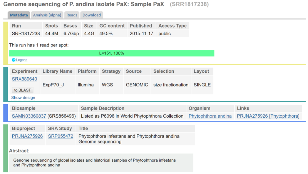
When talking to Lars Arvestad after the seminar, we were told that our data is not “the best data”, and that the assembly might not be fantastic. We looked at the data (see figure below) and could indeed see that it is single end-reads (while most assembler mention using paired-end or/and mate-pair reads).

Screenshot of the sequencing data web page.

We are not sure yet how this will affect our assembly, and my thinking is that we will have to experiment a bit with the options available for ABySS and see what gives a better or worse assembly. For example, we could experiment with different k-mer sizes. However, I think we need to decide whether if it is more important to have an assembly that covers most of the genome, or to have a very accurate assembly of a part of the genome. From what I have understood it, it will be a bit of a trade-off.

The data

Today I also downloaded the sequencing data, both the reads and the CHS-gene files, to my folder on Rackham (UppMax). However, the format of the sequencing data file was in .gz-format, and I could not find a way to unzip that file on Rackham. Therefore I downloaded it locally to my computer, extracted it, and uploaded the acquired .fastq-file back to my folder on Rackham. This took a while considering the size of the files, but now we could take a look that the content which was as expected. Below is an example of a read.

@SRR1817238.2 HWI-ST897:215:H0RT3ADXX:1:1101:1174:2066/1
ATGAAAGTCCGGAGGATTCGGAGGAGGCTCGAGCCGTTGATGACGCCTTGGAGGAGGACACACGACGGGCCTTGTCCCAGTCCCGATCTGAAGCCCGGCGA
AGATCCTTTCAACCCCGCCTCCACAAGTCGCTGGTACCGCCGGATCCGGG
+
:?BABDDFFFCF@FH<CGFGIEHIGGHFHDHDFEIFHIJCGHHHHDFFDEEAED=@D8?C?CB=BBDDDBDDDDD@@CDCD@CC<5>@BCACCCBD<@9@>
9>BCCCCCDCDDDDDDB@DBDB?CDDBDDDDDDB?CDCBDBBDDDBD<@#

Using the following command (and assuming there is not subsequent score of @SRR) the following total of number of reads can be counted:

grep -o '@SRR' SRR1817238.fastq | wc -l
44445500

Regarding the CHS-genes, I seems like we do not have permission to copy that file from where it is deposited at UppMax (/proj/g2017020/nobackup/Phytophthora_andina) to our own home directory. This means we can not view the data at the moment, but we will still be able to use it for example with BLAST directly on Rackham.

That’s it for now. Tomorrow we will try and assemble the genome.

In today’s meeting the presentation for tomorrow’s seminar was finalized.

We also made the first draft of our Gantt schedule and we will most likely revise it, especially now in the beginning when we are still researching the different options of how to solve the problems in this project. A screenshot of the Gantt schedule can be seen below.

Current Gantt schedule

Choosing the assembler

One of the first discussions we had as a group was regarding the type of assembler we will use for our genome assembly. As mentioned in a previous post, a list of all assemblers available on UppMax was made (42 assemblers in total!). Out of these 42 assemblers, 20 assembler options could be removed due to different reasons:

• They are made for RNA-seq data specifically, and not DNA which is what we have (e.g. Trinity or Trans-ABySS),
• They are specifically designed for handling long-read sequencing data (e.g. FALCON or canu), from for example PacBio, but we have short reads from Illumina.

Out of the 22 other assemblers, 7 was removed due to either being made for analyzing metagenomics data (and not specifically for assembling genomes de novo), analyzing massively parallel sequencing data, or simply not being documented well enough for us to understand what they do at this point. An important factor is after all that the tool one uses not only is suited for the type of project, but also that it is well-documented and that people “out there” are using it. If the tool is well-used for similar projects, then that indicates it is a good tool (or that it is the only one available, but now we know that is not the case).

Left was then 15 assemblers that from quick research seemed to be good options. We decided today to look into the following assemblers in more detail:

• ABySS (there is a version that assembles genomes > 100 Mb)
• SOAPdenovo
• Velvet

In the next-coming days, we will look specifically into what input and output these assemblers have, if they have scaffolding as a part of the assembly, and generally how accurate they seem to be. Additionally, the actual documentation and syntax for how to use the assemblers will be looked into so that we can start the assembly process!

To summarize our biggest questions at this point:

1. Once we have our first assembly, what are the best way of evaluating its accuracy?
2. How do we best compare the results obtained from different assemblers?
3. Why and how do we take out the largest contig from our genome of interest, and compare that to the reference genome (as instructed in the project)? Can one compare the whole genomes?

Project planning

At the first group meeting, all group members were present and the project background and aim was discussed to make sure everyone has understood what the project is about. The main goal of this meeting was to organise the work for the upcoming days before the presentation on Seminar 1 (30th of November). It was decided that all project work (except for the individual diaries) is documented using Google Suite tools, i.e. Google Docs, Google sheets and Google Presentation.

It was decided that an initial project plan, the Seminar 1 presentation, and basic read-up on assemblers and assembly approaches in general, should be done at the latest the evening of the 29th of November. An update on the presentation and project plan will be available in the next post.

Initial ideas for the project

As the main task is to assemble the genome of P. andina, we discussed different approaches and naturally what assembler we would use. A list of all assemblers available on UppMax was created and each assembler will be evaluated for the next coming 2 days in order to see which one fits the project best, and perhaps most importantly the data.

As the genome of the eukaryote P. infestans is around 240 Megabases (the largest genome of all known Oomycetes) we assume the genome of P. andina will be of similar size (being its closest relative). We discussed three main criteria that our assembler should fulfill:

• Be able to handle Eukaryotic genomes and all that comes with it, e.g. repetitive regions
• Handle short reads
• Handle medium-sized genomes (the genome is not huge, but not very small either).

Since we will have to annotate genes, BLAST is the first tool that comes to mind. We decided that we would already now look into how BLAST can be used for this task.

Background

Oomycetes is a group of Eukaryotic microorganisms that includes many different pathogens. One of these pathogens, Phytophtora infestans, is the most destructive pathogen of many different crops, in particular potato - an integral part of much of the world’s food supply. The species P. infestans and other Oomycetes are therefore important to study, and their ability to invade host species make the them interesting to study from an industrial perspective.

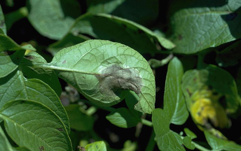
Potato leaflet infected by P. infestans. By Howard F. Schwartz, Colorado State University, United States

Several genes of oomycetes have been studies before, and specifically chitin synthase (CHS), an enzyme involved in building up the cell walls. In order to get a better understanding of these genes, the genome of the species of interest needs to be assembled, and the species on which we will focus is P. andina which has been proved to be a hybrid of P. infestans and other unknown Phytophtora species.

The data

In order to assemble the genome of P. andina, sequencing data is needed. Provided in this project is sequencing data deposited att UppMax (cluster-based super computer in Uppsala) including both Illumina reads and CHS genes.

The goal

Using the deposited sequence data, our goal is to assemble contigs based on the data, identify CHS genes and then compare these genes to those of P. infestans. Additionally, the aim is to compare the largest obtained contigs in the assembly, with the corresponding parts of the P. infestans genome published in 2009. Lastly, we aim to determine whether P. andina, as mentioned a hybrid between P. infestans and other Phytophtora species, can contribute with information to the study.

The following code snippet will greet the World. He is a nice guy.

  echo 'Hello Mr. World.'